This document is intended to help you learn more about fundamental machine learning concepts and how to best apply them to Qeexo AutoML projects in order to achieve the best result.

What is Machine Learning?

Machine Learning is an AI (artificial intelligence) technique that teaches computers to learn from experience. Machine Learning algorithms use computational methods to “learn” information directly from historical data without relying on a predetermined equation. It uses historical data as input to predict new output values. Similar to how humans learn and improve upon past experiences, the machine learning algorithms adaptively improve their performance as the number of samples available for learning increases.

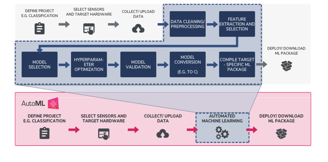
Traditional Machine Learning Workflow VS. Qeexo AutoML’s Fully Automated Machine Learning Workflow

There are multiple stages in developing a machine learning model for use in a software application. The typical phases include data collection > data pre-processing > model training and refinement > evaluation > deployment to production. When starting on a new machine learning problem, you first need to define the project, determining what you want the machine learning model to predict, once defined you can start working on solving the problem.

Qeexo’s AutoML’s fully automated machine learning workflows allow teams to be more efficient in finding the best performing model for their machine learning problem. Automating the most process intensive tasks from traditional machine learning processes, like data cleansing, sensor and feature selection, model selection, hyperparameter optimization, model validation, conversion, and deployment, Qeexo AutoML saves users time, and alleviates a number of challenges, by evaluating hundreds of options and determining which are best suited to learn from your data, all behind the scenes. This is so-called AutoML.

Best Practices for Efficient Workflows in Qeexo AutoML

Define your project / What do you want to predict?

Depending on your machine learning question, you project can be created with one of three different Classification Types: single-class anomaly classification, multi-class classification, and multi-class anomaly classification. Single-class anomaly classification applies when you intend to predict whether new, incoming data is normal or an outlier/anomaly. For example, predicting / monitoring whether a manufacturing machine is working normally or not. Multi-class classification applies when you intend to predict two or more discrete classes of events, for example, whether a robot arm is gripping a box, a bottle, or a bag. Multi-class anomaly classification can be thought of as a combination of the previous two classification types, where other than the learned classes, you also want to be able to predict any event or anomaly that doesn’t fall into the given classes.

Data collection

Data collection is a foundation of a machine learning project. During the data collection, the data quality can be defined as its volume, variety, and veracity. Ensuring your machine learning model has enough data to learn from, the data covers as much scenarios as possible, and data collected are accurate are critical for the performance of the model.

When you are collecting data in Qeexo AutoML, you will need to set up an environment by selecting sensors and corresponded Output Data Rate (ODR) and Full-Scale Range (FSR). ODR also known as sampling rate, is the rate at which the sensor obtains new measurements. ODR is measured in number of samples per second (Hz). Higher ODR configurations, typically specified in KHz, result in more samples obtained per-second. Higher ODRs can improve model accuracy since it provides more information during training and inference, however, for embedded applications, there may be memory, latency, and power consumption constraints that should be considered when specifying your sensor’s ODR. Users may want to test out different ODRs to figure out what will be the best option. Two sensors, which often have variable FSR settings, are accelerometers and gyroscopes. An Accelerometers’ FSR measures acceleration (rate of change of velocity of an object) in X, Y and Z directions, in the units of gravity (g). Gyroscopes’ FSR measures angular velocity in Degrees Per-Second (dps) in X, Y and Z rotational directions.

For a more detailed description of ODR and FSR, check out this post from the Qeexo Blog: ODR and FSR of Sensors

Data Segmentation

The Data Segmentation feature in Qeexo AutoML supports you in editing your data collections to your liking. If your data is event based, or a single data collection you recorded covers multiple different events and classes, it is helpful to use this feature to crop and label your data into individual, discrete events before training. Keep in mind the model will only learn from data that has been labelled and included in training, therefore cropping and labelling individual events helps the model better understand each class and filter outliers and noise which generally leads to improved model performance.

Model training settings

After selecting your data collections you will Start New Training, in Qeexo AutoML this means configuring your Sensor and Feature Selection, Inference Settings, and Algorithm Selection.

Deciding which sensors to use as input to your machine learning model is one of the most critical decisions you can make in solving a problem using sensors and tinyML. For example, if you are trying to recognize a type of motion – such as walk vs. run vs. rest – environmental sensors like temperature, humidity and pressure are probably not going to provide you with all of the data needed to distinguish between the three activities; however, sensors like accelerometer and gyroscope are specifically designed to help you recognize various types of motion, and are often the cornerstone of fitness tracking wearables like as FitBit. Inversely, trying to build an air quality monitor to detect harmful gasses in a factory using only accelerometers and gyroscopes would also likely not lead to optimal results, where environmental sensors such as gas, temperature, pressure, and humidity may provide sufficient information by which to make decisions about a factory’s air safety.

For Sensor and Feature Selection from Qeexo AutoML, there are two two options: automatic or manual. If you know which sensors matter to your ML question, then you may want to go with a manual configuration. However, if you are not sure, selecting the Automatic Sensor Selection option lets Qeexo AutoML test different groups of sensor selections and selects the best combination for you. We advise you to enable as many sensors as possible during the data collection stage and allow Qeexo AutoML to evaluate them for you.

For Inference Settings, there are two figures here – Instance Length and Classification Interval. Instance length is the duration of the incoming data that the software will use to make the prediction. Classification interval is the frequency at which the software will make each prediction. A longer Instance Length corresponds to a larger number of samples for featurization. More data points could yield finer frequency resolution, which captures an increased quantity of information from the signals. Therefore, it produces a greater number of features for the ML model training. Classification interval refers to the time interval in milliseconds between any two classifications. Classification interval is not optimized even when selecting the “Determine Automatically” option. Shorter intervals make predictions more frequent, but consume more power, while longer intervals save power, but can miss quick-burst live-streaming events when they occur between two consecutive classifications. When you have an event that happens in very short time duration, you may want to manually set your Classification Interval to a value smaller than your event duration.

Just like Sensor and Feature Selection, from Qeexo AutoML you can either choose Manual or Automatic Inference Settings. Similarly, choosing the automatic option means Qeexo AutoML will test different Inference Settings behind the scenes and choose the combination that yields the best performance. If you don’t have a solid figure in mind, it is suggested to try with the automatic option and twist it later to improve.

For a more detailed description of Inference Length and Classification Interval, check these two posts from the Qeexo blog: Inference Settings: Instance Length and Classification Interval and Classification Interval for Qeexo AutoML Inference Settings

Algorithms Selection

Qeexo AutoML supports up to 17 algorithms from the platform. If you don’t have a specific algorithm that you want to use, we advise you to enable all of them during training, and do a comparison. Once you click Next, the software will start running.

Below are some links that we recommend you check out if you’d like to learn deeper about ML algorithms: All Machine Learning Models Explained in 6 Minutes and Deep Learning in Qeexo AutoML Platform.

 How to check model performance?

Once training has completed, users have access to a model Performance Summary for each model from Model page. Here you will find a number of metrics useful in evaluating model performance including UMAP Plot, PCA plot, Confusion Matrix, Cross Validation, Learning Curve, ROC Curve, Matthews Correlation Coefficient, and F1 Score.

We are providing some explanation and tips below to help you better use some of these metrics to understand your model performance and where it can be improved.

Confusion Matrix forms the basis for many other metrics including ROC curve and F1 score, so it is critical to understand it first. The two images below may help you better understand what each value in the matrix means. The x-axis are the actual values of your data, whereas the y-axis are the values that your model predicted to be. As you can see from the image on the left, the top left or bottom right cells (in green color), when both actual value and predicted value match, it will show as True Negative or True Positive. Thus, the diagonal elements, starting at the top left, represent the correct classification, meaning you would like to see higher values in these cells. In contrast, the off-diagonal elements (in red color) represent misclassifications, meaning you would like to see smaller values here. If you are seeing a number of misclassifications you may want to try different actions to improve your model performance.

ROC Curve of a classifier is equal to the probability that the classifier will rank a randomly chosen positive example higher than a randomly chosen negative example. The greater the value (area under the curve), the better is the performance of the model.

A high F1 Score is useful where both high recall and precision are important. It tells you how precise your classifier is (how many instances it classifies correctly) and how robust it is (does it miss a significant number of instances). High precision but low recall may give you accurate results for obvious classes, but tends to miss many instances that are a bit more difficult to classify.

To understand F1 Score, user first need to know about precision and recall. Please refer confusion matrix for the meaning of TP (True Positive), TN(True Negative), FP(False Positive), FN(False Negative).

Matthews Correlation Coefficient: Is a measure of discriminative power for binary classifiers. In the multi-class classification case, it quantifies which combinations of classes are the least distinguished by the model. The values can range between -1 and 1, although most often in Qeexo AutoML the values will be between 0 and 1. A value of 0 means that the model is not able to distinguish between the given pair of classes at all, and a value of 1 means that the model can perfectly make this distinction.

For more detailed information about model metrics, please check out the link below:

Model Performance Evaluation in Qeexo AutoML

Testing Your Model

You have two ways to test your model performance from Qeexo AutoML. The first is to use the Test Data Evaluation feature with test data that has been upload or collected previously. Click the edit test data option > select the test data collection > and click SAVE to execute the test data evaluation. Once the build is complete, check your cross-validation accuracy and model performance summary as a gauge in how well your model would perform in the real-world given the data.

Another way to test your model’s performance is through Live Test. From Qeexo AutoML you can flash the machine learning model directly to your supported embedded device and perform real-time, on device classification to see how well you model performs. This has some advantages in that you may be able to find issues that are not easy to notice through the model performance summary, for example, misclassifications, flickering, classification delays / latency.

Here are some tips when you are seeing misclassifications, flickering, or delays during your Live Test. (1) If you did not collect data from all possible scenario, then you may see misclassifications / flickering when you conduct a Live Test, this is because your model has never learned about the new scenario’s data it just captured through live classification, but it has to pick a class from what it learned in the historical data and assign to it, then it may be a wrong representation. (2) If your data is not balanced, meaning some classes have much more data compared to other classes, then you may see a higher occurrence of the class that counts as the majority. (3) Cross validation is a good measure but Live Test may show a different result. We encourage you to live test on multiple models to find the best performing one for further improvement.

Actions You Can Take to Improve Model Performance

Data collections used for model training

If you are seeing misclassification and flickering in live classification, we advise you to go back to the data you used for model training and verify if your data classes are approximately balanced in proportion, if you have used sufficient data, and if you covered as many scenarios as possible.

If you are using accelerometer and gyroscope and your model yields low accuracy, we advise you to try collect a new data with a higher ODR, as this could result in more samples per second, thus a higher performing model. The smaller the FSR, the more sensitive the accelerometer / gyroscope will be to lower amplitude signals / angular motions. If you want the model to be more sensitive to more detailed movement, lower your FSR.

Twist model inference settings

If your initial model is not performing well and you notice that your data is quick-burst event type, we advise you to try to lower your classification interval as a high value may miss the event. If your event takes some time to finish, check your inference length and try to make sure the length is long enough to cover the whole occurrence of an entire event. For example, when a event is a process of griper gripping an object which takes about 2 seconds. You would want to set your inference length at least 2000ms to capture the entire movement.

Live classification analysis – re-compile library with selected weight

Sensitivity Analysis reflects on how sensitive the model is for classes under consideration. The primary objective of the sensitivity analysis is to make the ML model lean more towards certain class(es) than the other(s). Qeexo AutoML performs the sensitivity analysis using Class Weight. From the models page you can go to Live Classification Analysis to analyze the sensitivity of each class and update their influence on the model performance. Here you can edit class weights and ‘re-compile library with selected weight’. Once you update the selected weights, you can click SELECT on the page and PUSH TO HARDWARE for live classification with new class weights.

The bigger the weight is, the more sensitive the model is to that class. In other words, the model is more likely to output class with the higher weight. Even though you can assign a weight to each class, only the relative difference between the class weights matter. That is, for three-class classification, weights {1,1,1} will have the same effect as {3, 3, 3} because this simply means each class has equal weights.

For real-world applications, finding the right weights for each class is a matter of trial-and-error or some predefined human knowledge. Qeexo AutoML offers very efficient method to test with different class weights, quickly check the classification performance, and then push the newly determined class weights in order to perform the Live Test.

For detailed information about sensitivity analysis, please check the link: Sensitivity Analysis with Qeexo AutoML

Manual calibration for single-class models

The Single Class anomaly models just output a “score” between 0 and 1 for how likely it is that the new data point is an “anomaly.” The “threshold” where the model decides to classify as “anomaly” defaults to 0.5, but the user can tweak it through Manual Calibration to be 0.7 or 0.3, based on what they are seeing from Live Classification.

For more detailed information, please check the link: Anomaly Detection in Qeexo AutoML